J Biomed 2017; 2:78-88. doi:10.7150/jbm.17341 This volume Cite
Review
Multiparametric Analysis of High Content Screening Data
Karol Kozak1,2 ![]() , Julia Seeliger1, Tomasz Gedrange1
, Julia Seeliger1, Tomasz Gedrange1
1. Clinic for Neurology, Carl Gustav Carus Campus, Technische Universität Dresden, Fetscherstr. 74, D-01307 Dresden, Germany;
2. Department of Informatics, Wroclaw University of Economics, Komandorska 118-120, 53-345 Wrocław, Poland;
3. Department of Orthodontics, Carl Gustav Carus Campus, Technische Universität Dresden, Fetscherstr. 74, D-01307 Dresden, Germany.
Received 2016-8-25; Accepted 2017-4-9; Published 2017-4-28
Abstract

Cell-based High-Content Screening (HCS) using automated microscopy is an upcoming methodology for the investigation of cellular processes and their alteration by multiple chemical or genetic perturbations. The analysis of the large amount of data generated in HCS experiments represents a significant challenge and is currently a bottleneck in many screening projects. This article reviews the different ways to analyse large sets of HCS data, including the questions that can be asked and the challenges in interpreting the measurements. The main data mining approaches used in HCS, such as image descriptors computations and classification algorithms, are outlined.
Keywords: High-Content Screening, cellular processes, data mining
Introduction
Fluorescent microscopy has enabled multifaceted insights into the detail and complexity of cellular structures and their functions for well over two decades. As an essential prerequisite for a systematic phenotypical analysis of gene functions in cells at a genome-wide scale, the throughput of microscopy had to be improved through automation. HCS is defined as multiplexed functional screening based on imaging multiple targets in the physiologic context of intact cells by extraction of multicolour fluorescence information. Simultaneous staining in 3 or 4 colors allows the extraction of various parameters from each cell quantitatively as well as qualitatively such as intensity, size, distance or distribution (spatial resolution). The parameters might be referenced to each other, for example the use of nuclei staining to normalize other signals against cell number, or particular parameters might verify or exclude each other.
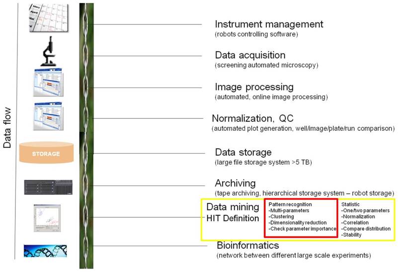
An essential factor in the success of high content screening projects is the existence of algorithms and software that can reliably and automatically extract information from the masses of captured images. Typically, nuclei are identified and masked first. Then, areas around the nuclei are determined or the cell boundaries are searched to mask the cell shape. For popular HCS assays at the sub-cellular level such as cell cycle analysis (mitotic index), cytotoxicity, apoptosis, micronuclei detection, receptor internalization, protein translocation (membrane to cytosol, cytosol to nucleus, and vice versa), co-localisation, cytoskeletal arrangements, or morphological analysis at the cellular level such as neurite outgrowth, cell spreading, cell motility, colony formation, or tube formation, ready-to-use scripts are available and need only some fine-adjustment for the particular cell line and/or conditions of the assay. Presently available analysis methodologies for large-scale RNAi (siRNA) data sets typically rely on ranking data and are based on single image descriptor (feature) or significance value 1, 2, 3. However, identifying patterns of image descriptors and grouping genes into classes based on multiparamteric analysis might provide much greater insight into their biological function and relevance (FIG 1). When determining whether a particular siRNAs is similar to control, there are four characteristics that need to be considered multiparametric analysis: absolute image descriptor value, or whether the siRNA signal (one descriptor) is at a high or low level; subtractive degree of change between groups, or the difference in descriptor across samples (calculated using subtraction); fold change between groups, or the ratio of descriptor across all samples (calculated by division); and reproducibility of the measurement, or whether samples with similar characteristics have similar amounts of the gene transcript. Classification techniques for comparing two sets of screening measurements essentially evaluate these four characteristics for each siRNA in various ways to rank siRNA that are most similar to controls.
Many free and commercial software packages (Table 1) are now available to analyse HCS data sets using classifiers, although it is still difficult to find a single off-the-shelf software package that answers all questions related to RNAi silencing. As the field is still young, when developing a bioinformatics analysis pipeline, it is more important to have a good understanding of both the biology involved and the analytical techniques rather than having the right software. This article reviews the different machine learning methods to analyse HCS data.
Dimension Reduction and Image Descriptors Selection
Mathematically, a HCS experiment with n (siRNA oligonucleotides) and represented by m (m >3) image descriptors is an n· m dimensional matrix. There is no way to graph the matrix, although one would like to review the diversity graphically. In order to solve this problem, dimensionality needs to be reduced to two or three. Dimensionality reduction should be a first preprocessing step in multiparametric data analysis. Many dimension reduction approaches are available. We will summarize some of the widely accepted dimension reduction technologies.
The key steps necessary for conducting a data flow of high-content image based screening. This HCS informatics pipeline consists of instrument management (logistic - booking systems), data acquisition using automated microscopy, automated image processing, normalization together with quality control, data storage using relational databases, archiving on tape storage system, data analysis including data modeling and visualization for hit definition and as last step bioinformatics. Highlighted parts in red color in this figure are our focus of discussion in this paper.
Some freely and commercial available software for HCS analysis. Although many bioinformatics companies sell software that assists in HCS analysis, there are several freely available software packages that can be used to perform the six analytical techniques described in this article.
| Name | Description | Source |
|---|---|---|
| CellMine Commercial | Integrates screening data with images and facilitates linkage to complementary discovery data and compound information. It unlocks the value of cell-based assays by facilitating improved lead selection and optimization. | http://www.bioimagene.com |
| AcuityXpress Commercial | Integration of image acquisition, image analysis and informatics. As a result, cell-by-cell multi-parametric results are automatically linked with the images and analysis results. | http://www.moleculardevices.com/pages/software/acuityxpress.html |
| Genedata Commercial | Supports quality control and analysis of interactively managed early-stage and large volume screening datasets. | http://www.genedata.com |
| LabView Commercial | Graphical data mining software. Open Source and arbitrarily customizable. Data aggregation, filtering, missing values | www.ni.com/labview |
| SciTegic (now Accelrys) Commercial | Data analysis and mining Data analysis and workflow management based upon graphical programming (visual scripting): components are visually arranged to protocols. Configurable components for chemistry, statistics, sequencing, text mining. | http://www.scitegic.com |
| Spotfire Commercial | Visual data mining, Visual and explorative data mining of large datasets. Guided analytics (guides predefined analysis workflows). Integrates computational services for R-project and S-PLUS1 and connects SAS files. | http://www.spotfire.com |
| Batelle Visua Commercial | Visual data mining Mining in multidimensional space with very large sets of numerical, categorical, chemical and textual data. Feature extraction (relativity tool), dimensionality reduction for visualization, intuitive user interface. | http://www.omniviz.com |
| Insightful Commercial | Statistical computing and graphics Extended features for robust and nonparametric regression, multivariate analyses, graphics, etc. Handles very large datasets. | http://www.insightful.com |
| Umetrics Commercial | Statistical computing and design of experiments products focus on multivariate analyses. Interactive and versions for batch modeling and analysis. | http://www.umetrics.com |
| MathWorks Commercial | Matlab1 and Simulink1 High-level language and environment for algorithm development, visualization, analysis and numeric computation. Runs on various platforms. | http://www.mathworks.com |
| Partek Commercial | Data mining, machine learning Various distance and similarity metrices, PCA (principle component analysis), clustering, NLM (Pattern recognition, classification and prediction capabilities with artificial neural networks and genetic algorithms | http://www.partek.com |
| Cluster and TreeView open source | for hierarchical clustering and viewing dendrograms software also creates self organizing maps and performs principal-components analysis. | http://rana.lbl.gov/EisenSoftware.htm |
| GeneCluster 2.0 open source | used for constructing self-organizing maps nearest neighbours and performs other supervised methods | http://www-genome.wi.mit.edu/cancer/software/genecluster2/gc2.html |
| RELNET open source | relevance networks written in Java | http://www.chip.org/relnet |
| CellHTS2 open source | implemented in Bioconductor/R to analyze cell-based high-throughput RNAi screens. analysis and integration of multi-channel screens and multiple screens. | http://www.dkfz.de/signaling/cellHTS/ |
| Weka open source | collection of all pattern recognition algorithms tools for data pre-processing classification, regression, clustering, association rules, and visualization | http://www.cs.waikato.ac.nz/ml/weka/ |
| R-project open source | Based upon S-language (Bell Laboratories). Used in statistical method-profiling and applications for generalized linear modeling, (nonparametric tests, nonlinear regression, classification, clustering, etc.) Open Source and arbitrarily customizable. | http://www.r-project.org |
| ScreenSifter open source | hit list and the visualization of biological modules among the hits Gene Ontology and protein-protein interaction analyses. visualization of screen-to-screen comparisons | http://www.screensifter.com |
Multidimensional scaling
Multidimensional scaling (MDS)4 or artificial neural network (ANN) methods are traditional approaches for dimension reduction. MDS is a non-linear mapping approach. It is not so much an exact procedure as rather a way to “rearrange” objects in an efficient manner, and thus to arrive at a configuration that best approximates the observed distances. It actually moves objects around in the space defined by the specified number of dimensions and, then checks how well the distances between objects can be reproduced by the new configuration. In other words, MDS uses a minimization algorithm that evaluates different configurations with the goal of maximizing the goodness-of-fit (or minimizing “lack of fit”)5.
Self-organising map (SOM)
A SOM is basically a multidimensional scaling method, which projects data from input space to a lower dimensional output space. Self-organizing map (SOM) is one of the ANN methods. Effectively, it is a vector quantization algorithm that creates reference vectors in a high-dimensional input space (one dimension - one image descriptor) and uses them, in an ordered fashion, to approximate the input patterns in image space. It does this by defining local order relationships between the reference vectors so that they are made to depend on each other as though their neighboring values would lie along a hypothetical “elastic surface” 6, 7, 8. The SOM is therefore able to approximate the point density function, p (x), of a complex high-dimensional (multiparamteric, image descriptors) input space, down to a two dimensional space, by preserving the local features of the input data. SOM belongs to classifiers and will be also describe later.
Supervised or Unsupervised
Current classification methodologies are based upon pattern recognition algorithms to analyse multiparametric image descriptors delivered from image processing (n • m dimensional matrix). It can be divided into two categories: supervised approaches, or analysis to determine genes that fit a predetermined pattern; and unsupervised approaches, or analysis to characterize the components of a data set without the a priori input or knowledge of a training signal. Many of these algorithms are also offered as part of various software free available solutions and software development kits (SDK) (Table 1).
Dissimilarity measure
As first step in classification is to make a distinction between dissimilarity measures (also known as 'metrics') used not for clustering but also used in classification algorithms (Table 2). A dissimilarity measure indicates the degree of similarity between two siRNAs in screening data set. A clustering method builds on these dissimilarity measures to create groups of features with similar patterns. A commonly used dissimilarity measure is Euclidean distance, for which each gene is treated as a point in multidimensional space, each axis is a separate image parameter and the coordinate on each axis is the value of that parameter. One disadvantage of Euclidean distance is that if measurements are not normalized, correlation of measurements can be missed, the focus being instead on the overall amount of image descriptors. A second disadvantage is that siRNAs that are negatively associated with each other will be missed. Another dissimilarity measure that is commonly used is the Pearson Correlation Coefficient, which is measured between two siRNAs that are treated as vectors of measurements. Once a dissimilarity measure has been chosen, the appropriate classification technique can be applied. Next sections describe the four commonly used classification techniques: unsupervised techniques — hierarchical clustering, self-organizing maps, relevance networks and principal-components analysis — and two commonly used supervised techniques — nearest neighbours and support vector machines.
Dissimilarity measures
| Dissimilarity measures |
|---|
| In any clustering algorithm, the calculation of a 'distance' between any two objects is fundamental to placing them into groups. Analysis of HCS data is no different in that finding clusters of similar siRNAs relies on finding and grouping those that are 'close' to each other. To do this, we rely on defining a distance between each image descriptor vector. There are various methods for measuring distance; these typically fall into two general classes: metric and semi-metric. |
| Metric distances |
| Intensive used is a Euclidean distance and less intensive used metrtics: Pearson correlation coefficient, Uncentered Pearson correlation coefficient, Squared Pearson correlation coefficient, Averaged dot product, Cosine correlation coefficient, Covariance, Manhattan distance, Mutual information, Spearman Rank-Order correlation, Kendall's Tau |
| Semi-metric distances |
| Distance measures that obey the first three consistency rules, but fail to maintain the triangle rule are referred to as semi-metric. There are a large number of semi-metric distance metrics and these are often used in HCS data analysis. |
Supervised methods
Supervised methods represent a powerful alternative that can be applied if one has some previous information (training set) about which siRNA are expected to cluster together. Supervised methods are generally used for two purposes: finding siRNAs candidates with image descriptors that are significantly different between groups of known siRNA (controls), and finding siRNAs that accurately predict a characteristic of the control. There are several published supervised methods that find siRNAs or sets of siRNAs that accurately predict image descriptor characteristics, such as distinguishing one type of cancer from another, or a metastatic tumour from a non-metastatic one. These methods might find individual siRNAs, such as the nearest neighbour approach, and/or multiple genes, such as decision trees, neural networks and support vector machines. This article will focus on the two more popular supervised techniques: nearest-neighbour analysis and support vector machines.
Nearest neighbours
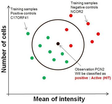
Although the nearest-neighbour technique can be used in an unsupervised manner, it is commonly used in a supervised fashion to find siRNAs directly with patterns that best match a designated query pattern (control). Given an input vector of image descriptors, nearest neighbor method extracts k closest image descriptor vectors in the reference set based on a similarity measure, and makes decision for the label of input vector using the labels of the k nearest neighbors (FIG. 2). Any metric can be used as the disimilarity measure. For example, an ideal siRNA pattern might be one that gives high number of cells as one parameter and low value of mean of intensity in second descriptor. Although this technique results in siRNAs that might individually split two sets of screening run, it does not necessarily find the smallest set of genes that most accurately splits the two sets. In other words, a combination of parameters of two siRNAs might split two conditions perfectly, but these two siRNAs might not necessarily be the top two hits that are most similar to the idealized pattern.
Support vector machines
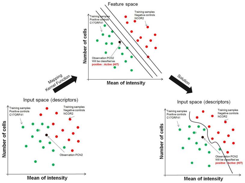
Support vector machines address the problem of finding combinations of siRNAs that better split sets of biological samples (wells in plate with siRNA). Although it is easy to find individual siRNAs that split two sets with reasonable accuracy owing to the large number of siRNAs (also known as features) measured on automated microscope, occasionally it is impossible to split sets perfectly using individual siRNAs. The support vector machines technique actually further expands the number of features available by combining siRNAs using mathematical operations (called kernel functions). For example, in addition to using the image descriptors of two individual siRNAs A and B to separate two sets of screening run, the combination features A *B, A/B, (A * B)2 and others, can also be generated and used. To make this clear, it is possible that even if siRNA A and B individually could not be used to separate the two sets of screening run, together with the proper kernel function, they might successfully separate the two. This can be visualized graphically as well, as shown in FIG. 3. Consider each plate well with one siRNA as a point in multidimensional space, in which each dimension is a one image descriptor and the coordinate of each point is the image descriptors value of that siRNA in the plate. Using support vector machines, this high-dimensional space gains even more dimensions, representing the mathematical combinations of siRNA. The goal for support vector machines is to find a plane in this high-dimensional space that perfectly splits two or more siRNA sets of screening run. Using this technique, the resulting plane has the largest possible margin from samples in the two conditions, therefore avoiding data over-fitting. It is clear that within this high-dimensional space, it is easier to separate siRNAs from two or more conditions (negative/positive/others), but one problem is that the separating plane is defined as a function using all the dimensions available.
Nearest-neighbour. The nearest-neighbour supervised method first involves the construction of hypothetical siRNAs that best fit the desired patterns. The technique then finds individual siRNAs that are most similar to the hypothetical genes.
Support Vector Machine. Instead of restricting to individual genes, support vector machines efficiently try several mathematical combinations of image descriptors to find the line (or plane) that best separates groups of siRNAs from screening run. SVMs use a training set in which genes known (controls) to be related by, for example function, are provided as positive examples and genes known not to be members of that class are negative examples. SVM solves the problem by mapping the image descriptor vectors from feature space into a higher-dimensional 'feature space', in which distance is measured using a mathematical function known as a Kernel Function, and the data can then be separated into two classes.
Unsupervised methods
Users of unsupervised methods try to find internal structure or relationships in a data set instead of trying to determine how best to predict a 'correct answer'. Within unsupervised learning, there are three classes of technique: feature determination, or determining siRNAs with interesting properties without specifically looking for a particular a priori pattern, such as principal-components analysis, cluster determination, or determining groups of genes or samples with similar patterns of image descriptors, such as self-organizing maps, k-means clustering and one- and two-dimensional hierarchical clustering and network determination, or determining graphs representing siRNA-siRNA or siRNA-phenotype interactions using Boolean networks 9, 10, 11, 12, 13, 14, This article will focus on the four most common unsupervised techniques of principal-components analysis, hierarchical clustering, self-organizing maps and relevance networks.
Hierarchical clustering
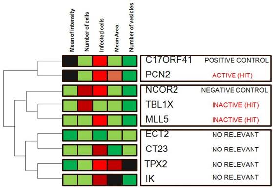
Hierarchical clustering is a commonly used unsupervised technique that builds clusters of siRNAs with similar patterns based on image descriptors. This is done by iteratively grouping together siRNAs that are highly correlated in terms of their image measurements, then continuing the process on the groups themselves. Dendograms (FIG. 4) are used to visualize the resultant hierarchical clustering. A dendrogram represents all genes as leaves of a large, branching tree. Each branch of the tree links two genes, two branches or one of each. Although construction of the tree is initiated by connecting genes that are most similar to each other, genes added later are connected to the branches that they most resemble. Although each branch links two elements, the overall shape of the tree can sometimes be asymmetric. In visually interpreting dendrograms, it is important to pay attention to the length of the branches. Branches connecting genes or other branches that are similar are drawn with shorter branch lengths. Longer branches represent increasing dissimilarity. Hierarchical clustering is particularly advantageous in visualizing overall similarities in image descriptor patterns observed in an experiment, and because of this, the technique has been used in many publications 15. The number and size of image descriptors patterns within a data set can be estimated quickly, although the division of the tree into actual clusters is often performed visually. It is important to note the few disadvantages in their use. First, hierarchical clustering ignores negative associations, even when the underlying dissimilarity measure supports them. Negative correlations might be crucial in a particular experiment, as described above, and might be missed. Furthermore, hierarchical clustering does not result in clusters that are globally optimal, in that early incorrect choices in linking genes with a branch are not later reversible as the rest of the tree is constructed. So, this method falls into a category known as 'greedy algorithms', which provide good answers, but for which finding the most globally optimal set of clusters is computationally intractable. Despite these disadvantages, hierarchical clustering is a popular technique in surveying image descriptor patterns in an experiment.
Hierarchical clustering. Genes in the demonstration data set were subjected to average-linkage hierarchical clustering using a Euclidean distance metric and image descriptors families that were colour coded for comparison. Similar genes appear near each other. This method of clustering groups genes by reordering the descriptors matrix allows patterns to be easily visualized. The length of the branch is inversely proportional to the degree of similarity. Shades of red indicate increased relative image descriptor; shades of green indicate decreased relative image descriptor.
Self-organizing maps
Self-organizing maps are similar to hierarchical clustering, in that they also provide a survey of image descriptors patterns within a data set, but the approach is quite different. Genes are first represented as points in multidimensional space. In other words, each biological sample (siRNA in well) is considered a separate dimension or axis of this space, and after the axes are defined, siRNAs are plotted using parameters (image descriptors) as coordinates. This is easiest to visualize with three or less siRNAs, but extends to a larger number of experiments/dimensions. Nearness can be defined using any of the dissimilarity measures described above, although Euclidean distance is most commonly used. The process starts with the answer, in that the number of clusters is actually set as an input parameter. A map is set with the centres of each cluster-to-be (known as centroids) arranged in an initial arbitrary configuration, such as a grid. As the method iterates, the centroids move towards randomly chosen genes at a decreasing rate. The method continues until there is no further significant movement of these centroids. The advantages of self-organizing maps include easy two-dimensional visualization of image patterns and reduced computational requirements compared with methods that require comprehensive pairwise comparisons, such as dendrograms. However, there are several disadvantages. First, the initial topology of a self-organizing map is arbitrary and the movement of the centroids is random, so the final configuration of centroids might not be reproducible. Second, similar to dendrograms, negative associations are not easily found. Third, even after the centroids reach the centres of each cluster, further techniques are needed to delineate the boundaries of each cluster. Finally, genes can belong to only a single cluster at a time.
Relevance networks
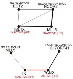
Continuing through the set of unsupervised techniques, relevance networks allow networks of features to be built, whether they represent siRNA, phenotypic or clinical measurements. The technique works by first comparing all image descriptors with each other in a pairwise manner, similar to the initial steps of hierarchical clustering. Typically, two siRNA are compared with each other by plotting all the samples on a scatterplot, using image descriptors values of the two siRNAs as coordinates. A correlation coefficient is then calculated, although any dissimilarity measure can be used. A threshold value is then chosen, and only those pairs of features with a measure greater than the threshold are kept. These are displayed in a graph similar to FIG. 5, in which siRNAs and phenotypic measurements are nodes, and associations are edges between nodes. Although the threshold is chosen using permutation analysis, it can actually be used as a dial, increasing and decreasing the number of connections shown. There are several advantages in using relevance networks. First, they allow features of more than one data type to be represented together; for example, if strong enough, a link between two image descriptors (number of cells and mean if intensity) of a particular siRNA could be visualized. Second, features can have a variable number of associations; theoretically, a transcription factor might be associated with more siRNAs than a downstream component. Finally, negative associations can be visualized as well as positive ones. One disadvantage to this method is the degree of complexity seen at lower thresholds, at which many links are found associating many siRNAS in a single network. Completely connected subcomponents of these complex graphs (known as 'cliques') are not easy to find computationally.
Principal-components analysis
PCA is used to transform a number of potentially correlated image descriptors into a number of relatively independent variables that then can be ranked based upon their contributions for explaining the whole data set. The transformed variables that can explain most of the information in the data, are called principal components. The components having minor contribution to the data set may be discarded without losing too much information. These dimension reduction approaches do not always work well. In order to validate the dimension reduction results, we need a technology to map a graphed point to its structure drawing.
Relevance networks. Relevance networks find and display pairs of siRNAs with strong positive and negative correlations, then construct networks from these siRNA pairs; typically, the strength of correlation is proportional to the thickness of the lines between siRNA, and red indicates a negative correlation.
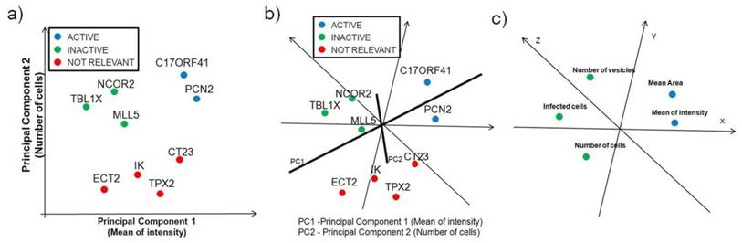
Principal-components analysis is more useful as a visualization technique. It can be applied to either siRNA or image descirptors, which are represented as points in multidimensional space, similar to self-organizing maps FIG 6a and FIG 6b. Principal components are a set of vectors in this space that decreasingly capture the variation seen in the points. The first principal component captures more variation than the second, and so on. The first two or three principal components are used to visualize the siRNA on screen or on a page, as shown in FIG. 6. Because each principal component exists in the same multidimensional space, they are linear combinations of the siRNAs. For example, the greatest variation of biological samples might be described as 3 times the particular image descriptor of the first siRNA, plus -2.1 times same descriptor of the second gene, and so on. The principal components are linear combinations that include every siRNA or image descriptor, and the biological significance of these combinations is not directly intuitive. There are other caveats in using principal components. For example, if screening runs are performed on samples from two conditions, principal components will best describe the variation of those samples, but will not always be the best way to split samples from those two conditions. Additionally PCA is a powerful technique for the analysis of screening data when used in combination with another classification technique, such as k-means, hierarchical clustering, or self organizing maps (SOMs) that requires the user to specify the number of clusters.
Principal Component Analysis. Principal-components analysis is typically used as a visualization technique, showing the clustering or scatter of siRNAs (or samples) when viewed along two or three principal components. In the figure c), a principal component can be thought of as a 'meta-biological sample', which combines all the biological samples so as to capture the most variation in image descriptors. Correlated parameters are close together, while anticorrelated parameters are in the other side of the origin. Principal components are showing the close correlation between the Mean Area and Mean of Intensity measurements.
Missing Values
Due to various effects during automated transfection, staining, and data analysis, not each siRNA can be assigned a meaningful ratio. HCS experiments often generate expression data arrays with some missing values. This results in missing values in the data matrix. To calculate distances, only elements represented in both vectors are used. If there is a missing value in one or both vectors, this dimension is not included in the distance calculation. This can lead to various problems:
The greatest problems occur, if the distance is not independent of the number of vector elements n, as it is the case for Euclidian distance (Table 2) for instance. Vectors with missing values are then differently weighted in comparison with vectors with no missing values. Let's say there are 3 siRNA:
- A siRNA-vector with all values valid
- A siRNA -vector with all values present but not equal to 1.
- A siRNA -vector with only one value equal to the corresponding value of siRNA 1
If vector 1 & 2 and 1 & 3 are compared, the following results are obtained:
- 1 & 2: They are not similar so the distance is greater than 0
- 1 & 3: Only values, which are present in both vectors, are used for the distance calculation, so the siRNAs are treated similarly, because the only comparison results in distance 0. But vector 1 and 3 could also be completely different...
For that reasons, missing values are difficult to handle. A few are usually no problem, but if there are too many in comparison to the number of vector-elements n, an arbitrary result can be expected. Missing data is one of the problems that preprocessing techniques need to deal with when analyzing HCS data. Many techniques, such as hierarchical and K-means clustering, are ill suited to analyze such problem spaces, as they require a complete data matrix to do the analysis. It is important to recognize the fact that such methods require a complementary preprocessing algorithm to fill in an estimate for the missing data. Various interpolation algorithms can be used for this purpose with varying degrees of success. These techniques can range from simple steps, such as filling the spot of the missing data with a zero (which is only partially effective for a very narrow range of classification algorithms) or row (gene) averaging, to using sophisticated interpolation techniques to fill in the missing data spots.
Conclusion
The 'list of genes' resulting from a HCS should not be viewed as an end in itself; its real value increases only as that list moves through biological validation, ranging from the numerical verification of results with alternative techniques, to ascertaining the meaning of the results, such as finding common promoter regions or biological relationships between the genes. There are a number of pattern recognition techniques to analyze HCS data. The simplest category of these techniques is based on individual gene analysis. Examples of these techniques are fold approach, t-test rule, and Bayesian framework. More sophisticated techniques include classification and clustering analysis methods described in this paper. The hypothesis behind using clustering methods is that “genes in a cluster must share some common function or regulatory elements. However, classifications based on clustering algorithms are dependent on the particular methods used, the manner in which the data are normalized within and across experiments, and the manner in which we measure the similarity. Although different techniques might be more or less appropriate for different data sets, there is no such thing as a single correct classification. Finally, the use of HCS in basic and applied research in drug discovery is only going to increase, but as these data sets grow in size, it is important to recognize that untapped information and potential discoveries might still be present in existing data sets (Table 3).
Downloadable large data sets of RNAi screening.
| Name | Description | Source |
|---|---|---|
| FlyRNAi | Screens carried out in the Drosophila RNAi Screening Center between 2002 and 2006. | http://flyrnai.org/cgi-bin/RNAi_screens.pl |
| DKFZ RNAi | Database contains 91351 dsRNAs from different RNAi libraries targeting transcripts annotated by the Berkeley Drosophila Genome Project | http://www.dkfz.de/signaling2/rnai/index.php |
| FLIGHT | FLIGHT is a database that has been designed to facilitate the integration of data from high-throughput experiments carried out in Drosophila cell culture. It includes phenotypic information from published cell-based RNAi screens, gene expression data from Drosophila cell lines, protein interaction data, together with novel tools to cross-correlate these diverse datasets | http://www.flight.licr.org |
| PhenoBank | Set of C. elegans genes for their role in the first two rounds of mitotic cell division. To this end, we combined genome-wide RNAi screening with time-lapse video microscopy of the early embryo | http://www.worm.mpi-cbg.de/phenobank2 |
| PhenomicDB | PhenomicDB is a multi-organism phenotype-genotype database including human, mouse, fruit fly, C.elegans, and other model organisms. The inclusion of gene indeces (NCBI Gene) and orthologues (same gene in different organisms) from HomoloGene allows to compare phenotypes of a given gene over many organisms simultaneously. PhenomicDB contains data from publicly available primary databases: FlyBase, Flyrnai.org, WormBase, Phenobank, CYGD, MatDB, OMIM, MGI, ZFIN, SGD, DictyBase, NCBI Gene, and HomoloGene. | http://www.phenomicdb.de/index.html |
| HTS DB | HTS DB is a high-throughput screening database contains data from several screening projects. Currently there are data relating to: 94 Small scale siRNA screens in human cell lines 18 Genome-wide siRNA screens in human cell lines 2 Genome-wide siRNA screens in drosophila cell lines 4 miRNA inhibitor/mimic screens | http://hts.crick.ac.uk/db/public/ |
| MitoCheck | RNA interference (RNAi) screens to identify all proteins that are required for mitosis in human cells, affinity purification and mass spectrometry to identify protein complexes and mitosis-specific phosphorylation sites on these, and small molecule inhibitors to determine which protein kinase is required for the phosphorylation of which substrate. MitoCheck is furthermore establishing clinical assays to validate mitotic proteins as prognostic biomarkers for cancer therapy. | http://www.mitocheck.org/cgi-bin/mtc |
| ZFIN | ZFIN serves as the zebrafish model organism database. The long term goals for ZFIN are a) to be the community database resource for the laboratory use of zebrafish, b) to develop and support integrated zebrafish genetic, genomic and developmental information, c) to maintain the definitive reference data sets of zebrafish research information, d) to link this information extensively to corresponding data in other model organism and human databases, e) to facilitate the use of zebrafish as a model for human biology and f) to serve the needs of the research community. | http://zfin.org |
| MGI | MGI is the international database resource for the laboratory mouse, providing integrated genetic, genomic, and biological data to facilitate the study of human health and disease. | http://www.informatics.jax.org |
Competing Interests
The authors have declared that no competing interest exists.
References
1. Boutros M, Kiger AA, Armknecht S. et al. Genome-Wide RNAi Analysis of Growth and Viability in Drosophila. Cells Science. 2004;303:832-835
2. Moffat J, Grueneberg D, Yang X, Kim S, Kloepfer A, Hinkle G, Piqani B, Eisenhaure T, Luo B, Grenier JA. Lentiviral RNAi Library for Human and Mouse Genes Applied to an Arrayed Viral High-Content Screen. Cell. 2006;6:1283-1298
3. Kittler R, Putz G, Pelletier L. et al. An endoribonuclease-prepared siRNA screen in human cells identifies genes essential for cell division. Nature. 2004;432:1036-1040
4. Cox TF, Cox MAA. Multidimensional Scaling. Chapman & Hall/CRC Press: Boca Raton. 2000
5. Multidimensional Scaling. http://www.statsoft.com/textbook/stmulsca.html#general
6. Kohonen T, Kangas J, Laaksonen J. SOM_PAK, The Self-Organizing Map Program Package available for anonymous ftp user at Internet site cochlea.hut.fi, version 1.2, November 1992.
7. Zupan J, Gasteiger J. Neural Networks for Chemists. John Wiley & Sons, Inc VCH. 1993
8. Bernard P, Golbraikh A. et al. Comparison of chemical databases: Analysis of molecular diversity with Self Organising Maps (SOM). Analysis. 1998;26:333-346
9. Liang S, Fuhrman S, Somogyi R. Reveal, a general reverse engineering algorithm for inference of genetic network architectures. Pac Symp Biocomput. 1998:18-29
10. Wuensche A. Genomic regulation modeled as a network with basins of attraction. Pac Symp Biocomput. 1998:89-102
11. Szallasi Z, Liang S. Modeling the normal and neoplastic cell cycle with 'realistic Boolean genetic networks': their application for understanding carcinogenesis and assessing therapeutic strategies. Pac Symp Biocomput. 1998:66-76
12. Friedman N, Linial M, Nachman I. et al. Using Bayesian networks to analyze expression data. J Comput Biol. 2000;7:601-620
13. Butte A, Kohane I. Biostatistical Genetics and Genetic Epidemiology. Fall Symposium, American Medical Informatics Association. 1999:711-715
14. Butte AJ, Kohane IS. Mutual information relevance networks: functional genomic clustering using pairwise entropy measurements. Pac Symp Biocomput. 2000:418-429
15. Pelkmans L, Fava E, Grabner H. et al. Genome-wide analysis of human kinases in clathrin- and caveolae/ raft-mediated endocytosis. Nature. 2005;436:78-86
Author contact
![]() Corresponding author: Prof. Karol Kozak <karol.kozakde>
Corresponding author: Prof. Karol Kozak <karol.kozakde>